Audio Fingerprinting

My project: audioplay

Basic Signal Processing Basics

Waves

When a note is played on the piano, the sound that emanates from the piano and reaches our ears is actually a wave. As soon as the piano hammer hits the string, the air surrounding the piano string vibrates i.e. areas of low air pressure and high air pressure are created. These vibrations travel throughout the air and causes our ear drums to vibrate, causing other ear components to send signals to the brain. These signals are interpreted as "sound". [1]

Fourier Transform

Any waveform can be broken down into its constituent sine and cosine waves (also called simple sinusoids), for which the terms frequency and amplitude are more well-defined. For example, the waveform below is pretty irregular, so it's difficult to observe any concrete properties by just looking at it. Luckily, the Fourier Transform decomposes the waveform into simple sinusoids, from which we can observe the various frequencies that make up the waveform.

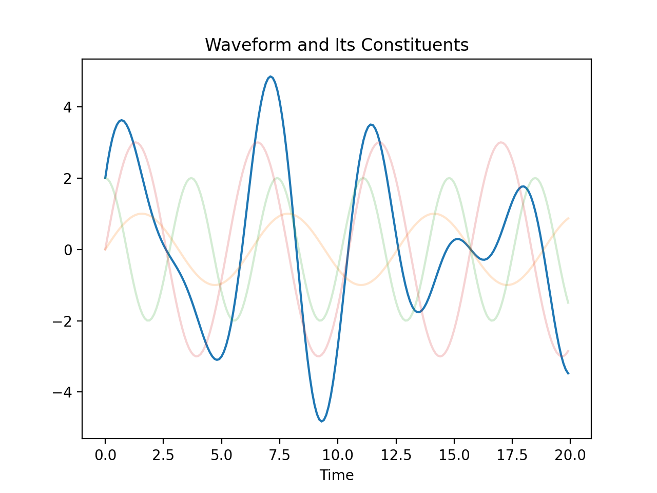
Notice how the faded orange, green, and pink waves are just simple sinusoids with uniform frequencies and waveforms. This is huge. The Fourier Transform implies that waveforms can be represented in terms of both time and frequency, each representation showing what the other cannot. [2] The canonical representation of waves is time-based, but notice that the temporal representation offers no obvious frequency information. On the other hand, the frequency representation likewise eliminates time information.

Digitalization

The above introduced the necessary tools and information for audio fingerprinting. However, music in its digital form places critical restrictions on these tools - as always, knowing when not to apply certain tools is just as important as knowing when to apply them, so we explore the relevant consequences of digitalization below.

Sampling and its consequences

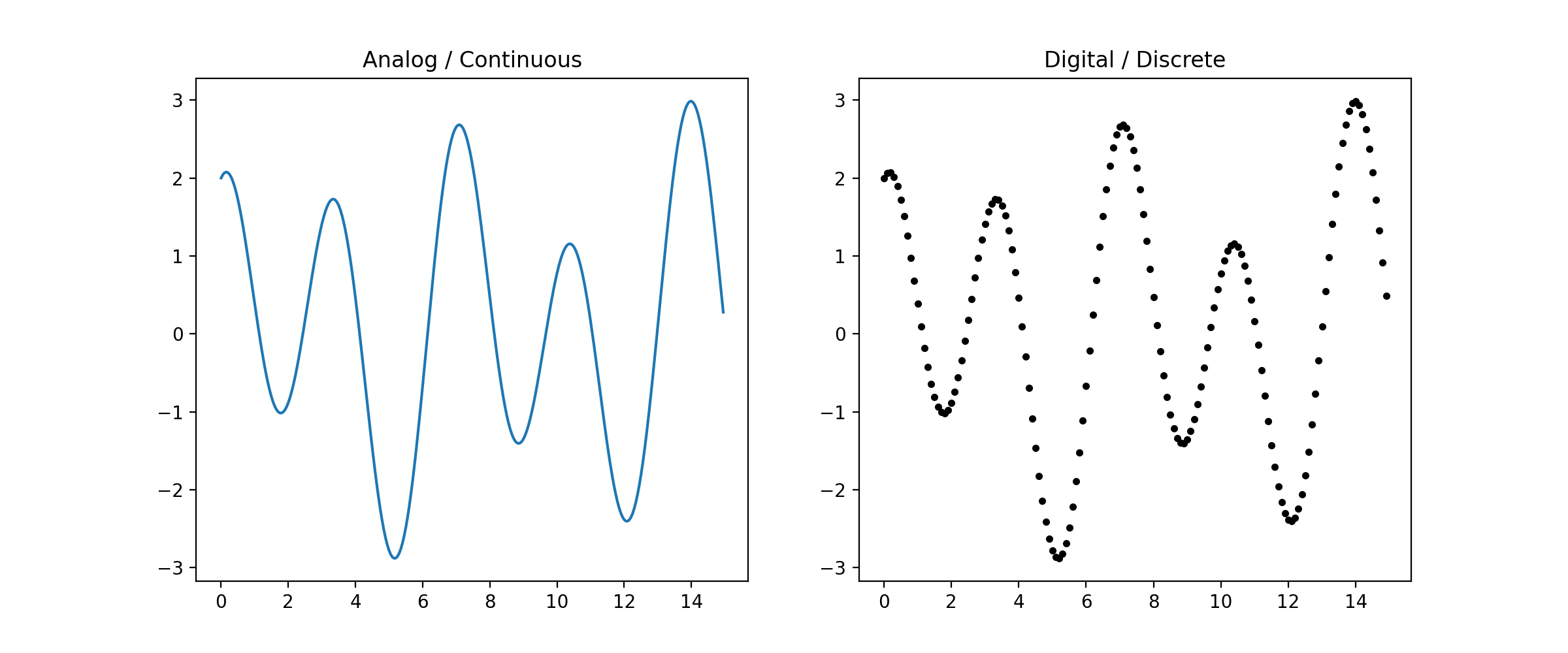
The difference between analog and digital music may be slight for the casual music listener, but most audiophiles will acknowledge that analog music sounds warmer and deeper compared to its counterpart - this is due to the process in which analog music is converted to digital music, or sampling. Sampling transforms a continuous signal into a discrete one. [3] As a simple illustration, making a connect-the-dots puzzle from a line drawing is essentially sampling - a conversion from the continuous to the discrete.

The specific mechanics of sampling consists of marking dots on a continuous signal at a fixed speed (called the sampling rate). But how fast should the sampling rate be such that the continuous signal can be deduced from its discretized form? We should hope that it's fast enough so that the deduction is easier than completing a connect-the-dots puzzle. A slow sample rate keeps us guessing, but a fast sample rate clearly shows the shape of the continuous signal.

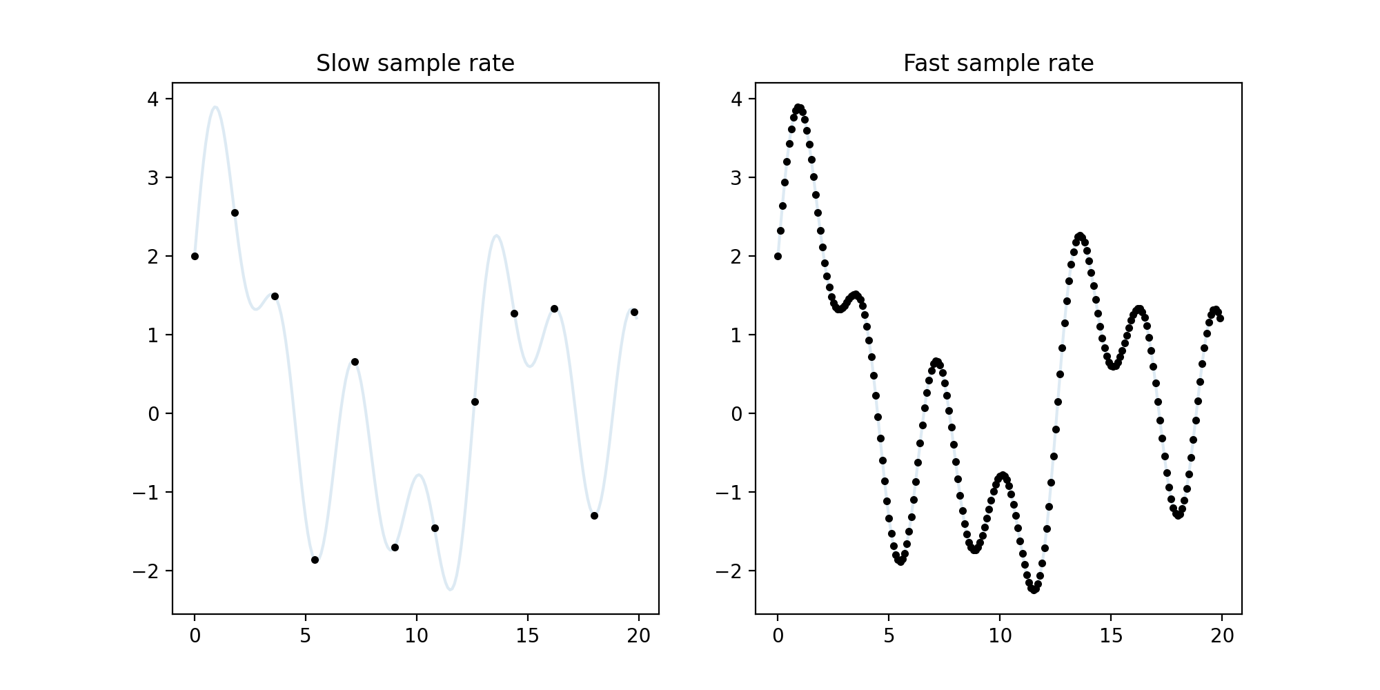
However, as the sample rate increases, the memory demand also increases. We're faced with a clear dilemma here: either increase the sample rate and risk taking up too much memory, or decrease the sample rate and lose data to the point that the original signal is impossible to deduce. Where is the Goldilock's zone of sampling rates for music?

The Nyquist-Shannon sampling theorem states that given a signal that contains no frequencies greater than \( B \) hertz, a sample rate of at least \( 2B \) samples per second is sufficient to reconstruct the continuous signal from its discretized form. Since human ears can only hear up to around 20 kHz, a sample rate of 40 kHz should be sufficient. This is where the magic number of 44.1 kHz comes from.

It seems as though we have resolved our digitalization problem. Sampling at 44.1 kHz is sufficient, so now we should be free to analyze digital waveforms. Unfortunately, the Fourier Transform in its current form poses a major obstruction.

Discrete Fourier Transform (DFT)

The Fourier transform can extract frequency information only from continuous waveforms. Luckily, a discrete version of the Fourier Transform exists, the aptly-named Discrete Fourier Transform. Without going into too much technical detail, the DFT essentially bins frequency information. The frequencies that the DFT extracts are grouped together; the exact specifications of these groupings is determined by the sampling rate and the window. We skip the technical details in this layman's introduction.

audioplay: reverse-search

As an exercise, let's explore what is important in song identification. As studied above, the essential components of any song are frequency, time, and amplitude.

• Amplitude. Clearly, the loudness (a.k.a. amplitude) is irrelevant; a song played at 10 dB is still the same song when played at 100 dB.
• Frequency. A song pitched up several semitones is noticeably different from the original song, so frequency should be important. Of course, the original song will be recognizable, but to say that the pitched-up version is the same as the original would be a stretch.
• Time. Similarly, a sped-up song is not the same as the original. However, overall song length is generally useless; instead, the time differences between specific moments are meaningful identifiers. For example, if a note hits earlier than you expect, then you will probably second-guess your memory.

With these ideas in mind, the project consists of two components: fingerprinting and recognition. The first transforms sound into a common medium that we can work with, and the second pertains to the song identification itself. In other words, fingerprinting is the mise en place, while recognition is the actual cooking.

The project's general overview is as follows:

1. Fingerprinting
• Spectrogram generation
• Peak detection
• Peak association
• Hashing
2. Recognition
• Fingerprinting
• Scoring

Fingerprinting

I. Spectrogram generation

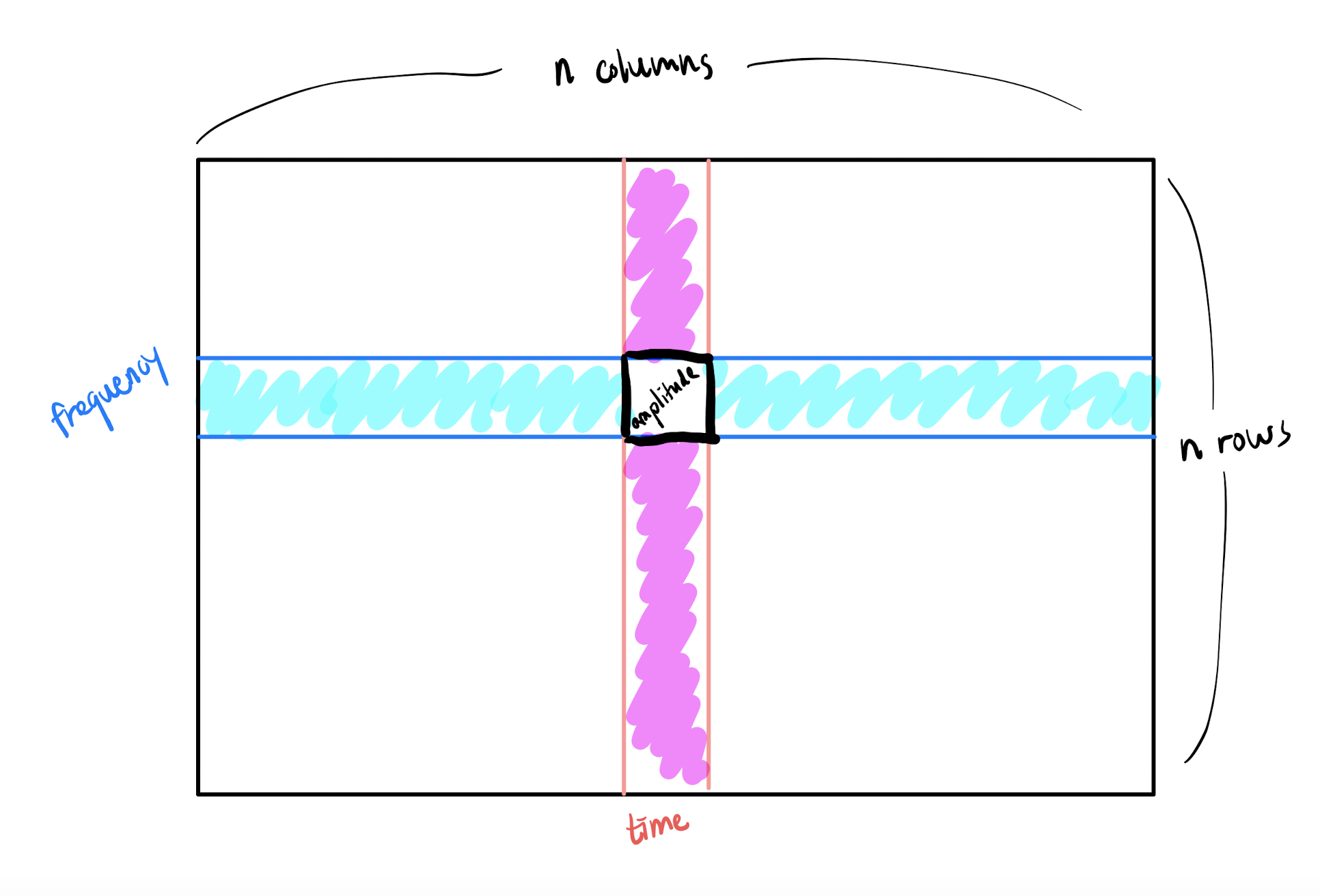
The spectrogram combines time and frequency information into a single representation, hence returning the time information lost through the Fourier transform. Because it compresses all the necessary information of a song into a single representation, it is the focal point of the entire fingerprinting process.

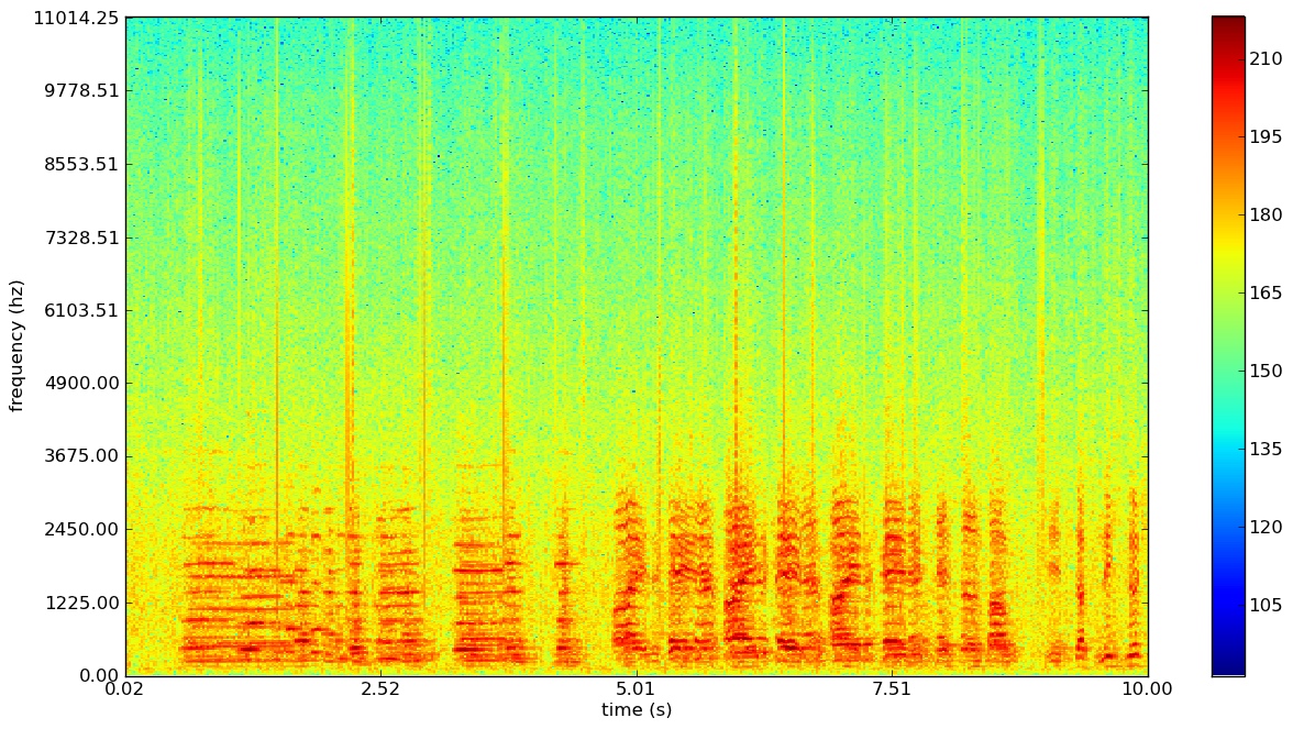
The x-axis, y-axis, and the color show the time, frequency, and amplitude, respectively. Just for intuition, notice that the above spectrogram shows red spikes, where nearly all the frequencies in the entire range are firing off at a high amplitude (this is probably the snare of the song). [4]

II. Peak detection

For our purposes, the spectrogram is an image, and an image is just an \(n \times n\) array of numbers, where each pixel is a cell in the array. The time and frequency determines the cell's location, and the amplitude dictates its value. A peak is then a (time, frequency) pair with the greatest amplitude value among the pixels surrounding it.

To identify peaks, we use binary morphology. [5] The process is as follows:

1. Place a 19-by-19 pixel square \(S\) over any part of the image.
2. Identify the pixel with the maximum value within \(S\). Call this maximum value \(M\).
3. Set all the pixel values within \(S\) to \(M\).
4. Apply the following rule to every pixel in \(S\): for any pixel \(P\) in \(S\),
   • If \(P = M\), color the pixel white.
   • If \(P \neq M\), color the pixel black.

For example, executing steps 1 through 3 gives the "Mask Applied" image [6], and the last step produces the "Identified Peaks" image. In the "Mask Applied" image, there are distinct squares, which are the 19-by-19 pixel squares described above. The "Identified Peaks" image shows scattered white dots on a black background, where the white dots are the maximal value pixels.

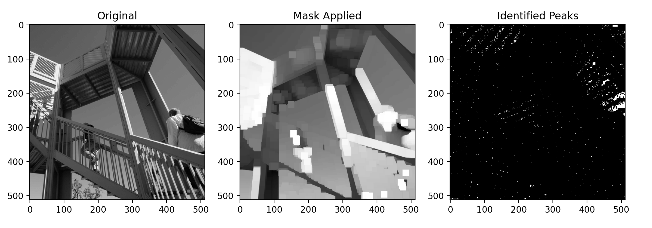
Finding the peaks is then just a matter of gathering the locations i.e. (time, frequency) pairs of the white dots. You may notice that by identifying peaks, we've lost all amplitude information, since the white dots show only the locations of the peaks. Thankfully, amplitude is not important for our purposes.

III. Peak Association

Surprisingly, this list of peak locations is actually sufficient for our goal to "reverse-search" audio. But we are greedy. Search needs to be fast, and using the vanilla list of peak locations would take absurdly long. By associating peaks with each other, we get higher information density and easy searchability at the expense of more computation. Not a bad deal.

The intuition behind peak association follows from the principle that the number of links between things increases faster than the number of things themselves. For example, there is only 1 possible link between 2 things, but 45 possible links between just 10 things.

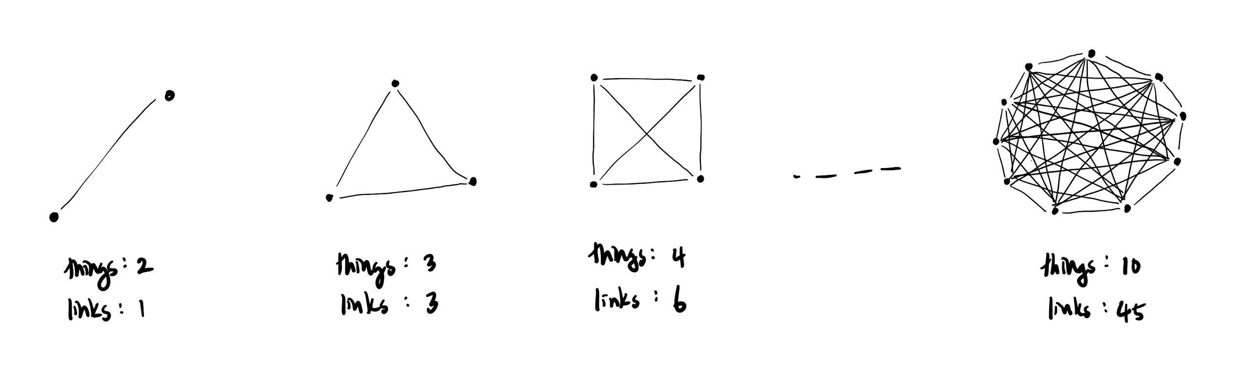
This means that from just a list of 10 peaks, we can extract 4 times as much information. The bang for our buck increases quadratically too, so more peaks means higher information density.

III-a. Anchors + Target Zones

However, chaotically pairing all possible peaks won't be fruitful - we need order in the chaos to extract the most information possible. The pairing method is as follows:

1. Order the peaks by time.
2. Choose a peak, and call it the anchor \(A\).
3. Choose the target peaks by selecting the 10 consecutive peaks \(\{ T_1, ..., T_{10} \}\) that come after skipping the first 3 peaks that are immediately after \(A\). For example, if \(A\) is the 10th peak, then the target peaks are the 14th, 15th, ..., 23rd peaks.
4. Form the pair associations \( \{ (A, T_1), ..., (A, T_{10})\}. \)
5. Repeat by setting every peak as the anchor, insofar as the 10 target peaks exist. For example, if only 10 peaks exist, then the 10th peak cannot be an anchor peak because there are no more potential target peaks.

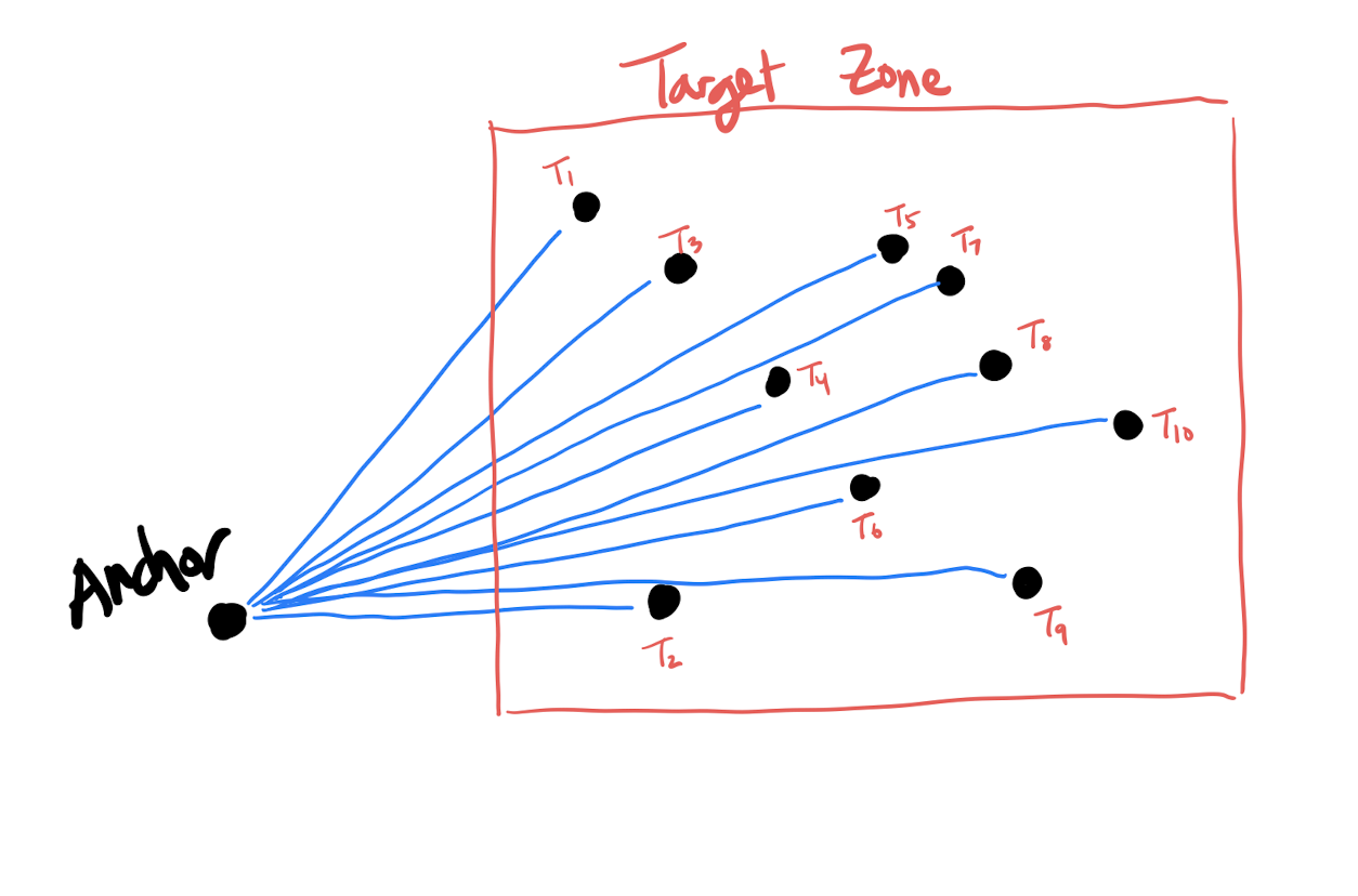
The anchor point brings order to the chaos. Because every peak in the target zone is linked to a common anchor point, every target peak has a "common denominator". In terms of ease of information access, there is a stark difference between saying "John is friends with Anne, Bob, and Clark", versus "Anne is friends with Bob, Clark is friends with John, etc".

IV. Hashing

Unfortunately, this list of peak pairs isn't easily searchable, so we need a method to compress each pair into an easily searchable form. Hashing associates each pair with a unique string, akin to how license plates uniquely identify cars. Input an anchor-target pair into the hashing function, and out comes a string that uniquely identifies that pair.

Recall that we hypothesized that only time difference and frequency are essential for identification. While the specifics of the hashing function aren't important, what we input into our hashing function reflects our hypothesis.

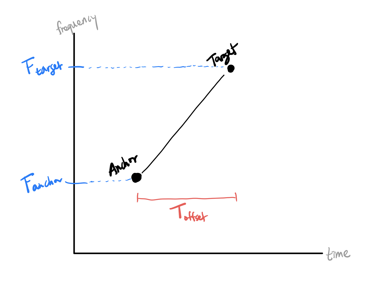
Remembering that every peak is a (time, frequency) point, for every anchor-target pair \( (A, T) \), identify:

• \(F_{\text{anchor}} := \) frequency of anchor peak.
• \(F_{\text{target}} := \) frequency of target peak.
• \(T_{\text{offset}} := \) time difference between target peak and anchor peak.

The triple \( (F_{\text{anchor}}, F_{\text{target}}, T_{\text{offset}}) \) becomes the input. By hashing every anchor-target pair, we generate a list of strings that uniquely identifies the song and is easily searchable. Having effectively translated music into organized, searchable data, this concludes the fingerprinting process.

Recognition

The sous chef has mise en place-d all the ingredients, and now it's time to cook. For the rest of this section, assume that we have a database full of song fingerprints. Also, we refer to the audio clip that needs to identified as the "id clip", and the database songs as the "db clips". For example, we need to check if the id clip matches any of the db clips.

I. Fingerprinting

Fingerprinting translates sound into a standardized form of data, so an audio clip must first be fingerprinted before recognition so that the clip can be analyzed. Fortunately, the same fingerprinting algorithms can be used for this stage, so nothing extra needs to be added.

II. Scoring

As an exercise, let's study how similar the fingerprints generated from two different sources playing the same song are. Both sources should generate similar spectrograms, and hence similar peaks. Therefore, the anchor-target pairs should coincide, with the only possible dissimilarities being in time and amplitude. Nonetheless, the time differences between the anchor-target pairs in both should be constant. In sum, the invariant information consists of the anchor-target pair frequencies and time differences, which are exactly the inputs of the hashing function.

Therefore, if the song in an audio clip matches a song in the database, then the hashes must coincide. Then identification simply becomes a matter of choosing the song that has the highest number of hash matches, and we are done! [7]

References and Further Reading

1. The original Shazam paper.
2. Will Drevo's dejavu project was invaluable and I heavily borrowed from the project source code.
3. Cameron Macleod's abracadabra also helped a lot.