A page from my research journal

I haven’t seen any blog posts about the process of training transformers. This is a page from my research journal: trying to get a from-scratch transformer to do what I want it to do.

Confusion 1: Data generation

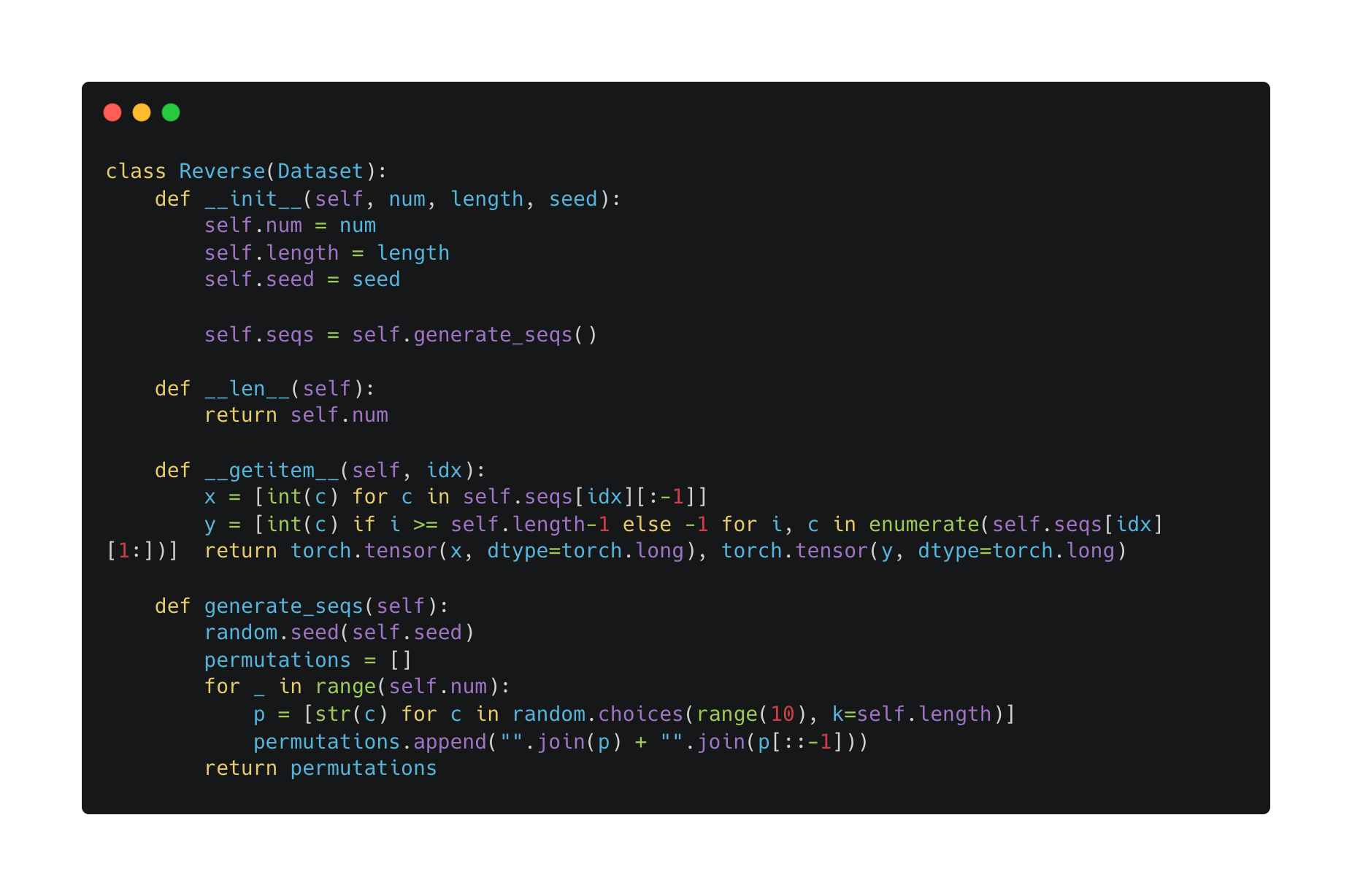
In order to check that I had set up masking correctly, I decided to train the transformer to reverse a sequence of digits. For example, given a sequence \((1, 2, 3, 4)\), I should get \((4, 3, 2, 1)\). But how should I set up the training data i.e. what should \(x\) and \(y\) be? I flipped through Andrej Karpathy’s minGPT to find out.

Turns out, in the example of \((1, 2, 3, 4)\), \[\begin{aligned} x &= (1, 2, 3, 4, 4, 3, 2)\\ y &= (-1, -1, -1, 4, 3, 2, 1) \end{aligned}\]

This is because the transformer is trained to predict the next token, at all the positions in the input. The \(-1\)’s in the target point indicate the tokens that should be ignored in the cross-entropy loss. We only care about reversing the sequence of digits, not about predicting the next digit in the given sequence.

The relevant code:

Confusion 2: Socrates data

Now it was time to get training on the Socrates data. I had several concerns at this stage.

1. How do I tokenize the Socrates data? I had seen the basics of tokenizers before, so a quick glance at the OpenAI tiktoken repository revealed how to encode and decode tokens. However, I still had to figure out the vocab size for the tiktoken GPT-2 tokenizer (otherwise, IndexErrors might crop up during the initial embedding step). After some snooping around, I found out that the GPT-2 byte-pair encoder (BPE) has a vocab size of 50,927.[1]

[1] Thanks HuggingFace!

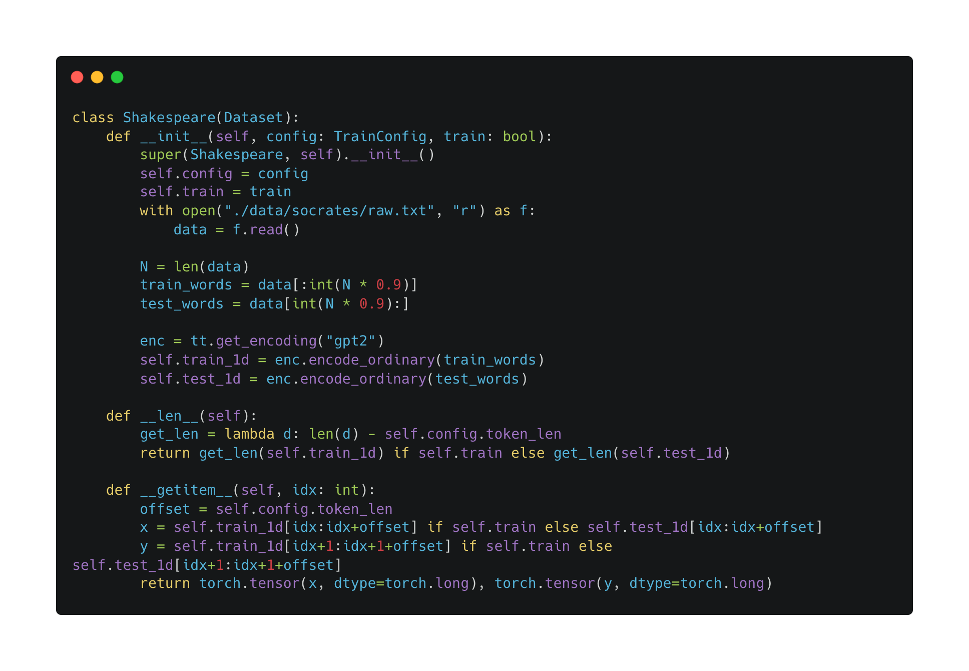
2. What should \(x\) and \(y\) be? Unlike the reverse-sequence task, no tokens have to be ignored for the Socrates task. For example, suppose the byte-pair encoding for “Socrates: I dare say that you may be surprised to find” is \((1, 2, 3, 4, 5, 6, 7, 8, 9, 10, 11)\). Then \[\begin{aligned} x &= (1, 2, 3, 4, 5, 6, 7, 8, 9, 10)\\ y &= (2, 3, 4, 5, 6, 7, 8, 9, 10, 11). \end{aligned}\] We want to train the transformer to predict the next token at every given position.

3. How should I write the Dataloader? After figuring out what \(x\) and \(y\) should be in the training data, writing the Dataloader was relatively simple. The relevant code:

Confusion 3: Coaxing pseudo-Socrates to overfit

I first did the stupid thing and pumped the entire Socrates dataset through the transformer at every epoch, and waited for an extremely long 10 epochs. However, the loss was barely going down! After each epoch, the average training loss was going down inconsistently by around \(2 \times 10^{-6}\).

I then did another stupid thing: I increased the learning rate, pumped the entire Socrates dataset through the transformer, and waited for another long 10 epochs. Again, the loss barely changed. Believe it or not, I went back to the learning rate and changed it five more times - with no improvement in loss degradation, of course. “Maybe adding a learning rate scheduler or using a different descent algorithm will help,” I thought. I added a learning rate scheduler and switched the descent algorithm from stochastic gradient descent to Adam. Did I expect there to be improvements? Frankly, yes. But wrong I was again - ninety minutes had gone by at this point.

I finally landed on the smart thing to do: go trivially small! Don’t train the transformer on the entire dataset, and instead train repeatedly on the same datapoint. If the model overfits (i.e. the validation loss has U-shape while the training loss continues to decrease), then the model is working correctly. Otherwise, either the model is hopelessly under-powered, or there is a bug in the code. I first beefed up the model parameters to make sure that my model was expressive enough. Then I removed the learning rate scheduler and set the learning rate to \(0.1\). “There,” I thought, “it should overfit now” - all I had to do was start training, and watch the magic.

No magical sparks flew - the loss barely moved! I suspected that the loss was not being propogated to the model, so I re-checked the PyTorch documentation for cross-entropy loss. Lo and behold:

I removed the last softmax layer, and hit train again. Still, the loss did not decrease.

I thought about the model from front-to-back: first, a single data point gets forward propogated through the model - then the loss is calculated - then the loss information is propogated backwards, and the whole cycle starts over again. I had dealt with the latter two steps - was there something wrong with the first? I checked my DataLoader code, and found the critical bug: I was shuffling the DataLoader at every step, so I was feeding in different points to the model! I quickly cooked up a debug flag that prevented the DataLoader from shuffling at every call.

Hands clasped in prayer, I hit train again, and got the following curves:

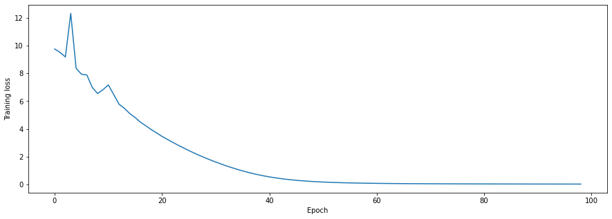
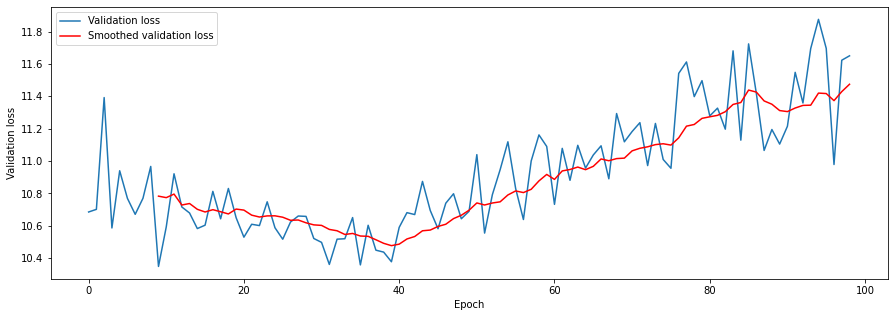
Thus we conclude this confusion stage with three important lessons:

1. Read the documentation.

2. When debugging, reduce - reduce - reduce to the trivial case.

3. When debugging machine learning models, remove as much randomness as possible! This is akin to statistical exercises - it’s imperative to keep track of which variables are stochastic and which are deterministic.

Confusion 4: Training pseudo-Socrates

With no outright bugs present in the code, I turned to actually training the transformer. I realized that I had zero clue of how machine learning optimization algorithms actually work; having taken a machine learning class, I knew about stochastic gradient descent and momentum, but the details behind fancy (?) methods like Adam were unbeknownst to me. Nor did I know in-depth about regularization methods.

This journey resulted in my deep learning optimization glossary.

With the newfound knowledge, I played with the learning rate and the batch size, and tried out different regularization methods like early stopping and dropout.

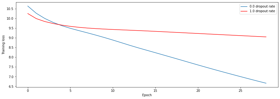
For a concrete example, check out the experiment that I tried to see the effects of dropout rate. Intuitively, the effective complexity of the model should increase as the dropout rate decreases. If the dropoput rate is 0.0, then all the units are always included. On the other hand, if the dropout rate is 1.0, then all the units are always zeroed out. Because I added dropout layers after having finished the base transformer code, I decided to run some trivial overfitting checks: if the model with maximum dropout rate learns better than the one with the minimum dropout rate, then something must be wrong. Indeed, the empirical results match with the intuition:

Confused, but now less so

My final model has ~17.7 million parameters, run with the Adam optimizer with initial learning rate 1e-3. Trained just under three hours on my MacBook CPU, it achieves a loss of ~0.37. Here are some generations, prompted with Socrates text:

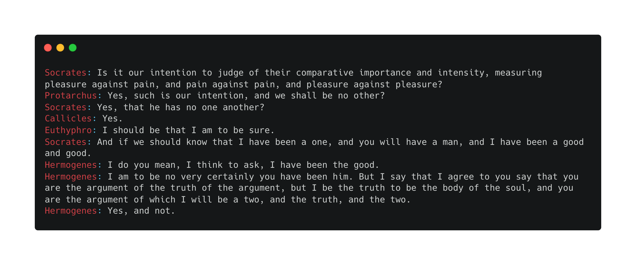
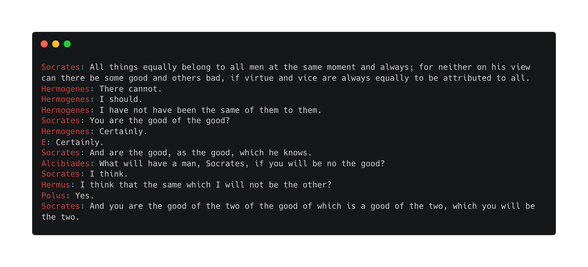Not good, but also not bad.

Appendix: Transformer Architecture

Decoder-only transformers have a pretty simple architecture. I’ve put a brief outline below.

Single-head transformers take an input and trace the steps written below. Note that all the vectors here are row vectors, because for some reason the machine learning community enjoys row vectors more than column vectors:

1. Take an input vector \(x \in \mathbb{R}^n\). Let \(e'(x) \in \mathbb{R}^{n \times d}\) be the embedding of \(x\), and \(p'(x) \in \mathbb{R}^{n \times d}\) be the positional encoding of \(x\).

2. Use \(e_x = e'(x) + p'(x)\) as the final embedding of \(x\).

3. Define \(q(x), k(x), v(x) \in \mathbb{R}^v\) as the query, key, and value vectors of \(x\), respectively. More specifically, we can define \[\begin{aligned} q(x) = e_x W_Q, k(x) = e_x W_K, v(x) = e_x W_V, \text{ where } W_Q, W_K, W_V \in \mathbb{R}^{d \times v}. \end{aligned}\]

4. Define the attention function \[\begin{aligned} A_{W_Q, W_K, W_V}(x) = \text{softmax}\left(\frac{q(x) k(x)^T}{\sqrt{v}}\right) v(x). \end{aligned}\] Notice that the attention function is parametrized by the query, key, and value matrices.

5. Project \(A_{W_Q, W_K, W_V}(x)\) back into \(d\)-dimensional space with the matrix \(W_O \in \mathbb{R}^{v \times d}\) i.e. take \(A_{W_Q, W_K, W_V}(x) \cdot W_O\).

6. Define \(l_{11}(x) = \text{LayerNorm}(e_x + A_{W_Q, W_K, W_V}(x) \cdot W_O)\).

7. Push \(l_{11}(x)\) through a feedforward neural network with ReLU activation to get \[\begin{aligned} l_{12}(x) = \max(0, l_{11}(x) W_1 + b) W_2 + b_2, \end{aligned}\] where \(W_1 \in \mathbb{R}^{d \times h}, W_2 \in \mathbb{R}^{h \times d}\) and \(h\) is the hidden layer dimension.

8. Define \(l_{1}(x) = \text{LayerNorm}(l_{11}(x) + l_{12}(x))\).

9. Repeat steps 3 through 7 for \(k\) layers. Denote the final output as \(l_k(x)\).

10. Project \(l_k(x)\) to the vocab size dimension i.e. take \(l_k(x) W_{\text{vocab}} + b_{\text{vocab}}\), where \(W_{\text{vocab}} \in \mathbb{R}^{d \times \text{vocab size}}, b \in \mathbb{R}^{\text{vocab size}}\).

11. Take the softmax to get \(y = \text{softmax}(l_k(x) W_{\text{vocab}} + b_{\text{vocab}})\).

Multi-head attention isn’t much different - we just need to numerate our query, key, and value matrices. Assuming \(h\) heads, we define \[\begin{aligned} q_i(x) = e_x W_Q^i, \text{ }k_i(x) = e_x W_K^i, \text{ }v_i(x) = e_x W_V^i. \end{aligned}\]

Then our attention function becomes \[\begin{aligned} A_{W_Q^i, W_K^i, W_V^i}(x) = \text{softmax}\left(\frac{q_i(x) k_i(x)^T}{\sqrt{v}}\right) v_i(x). \end{aligned}\]

To do step 5, we take \(W_O \in \mathbb{R}^{(h \cdot v) \times d}\), and apply it to the concatenated matrix to get \[\begin{aligned} \begin{bmatrix} A_{W_Q^1, W_K^1, W_V^1}(x) \mid & \cdots & \mid A_{W_Q^h, W_K^h, W_V^h}(x) \end{bmatrix} W_O. \end{aligned}\]